
MATLAB、Python、Scilab、Julia比較ページはこちら
https://www.simulationroom999.com/blog/comparison-of-matlab-python-scilab/

はじめに

の、
MATLAB,Python,Scilab,Julia比較 第4章 その89【ユニット数増加④】
を書き直したもの。
隠れ層のユニット数を増やすことで局所最適解にハマる現象を回避してみる。
今回はScilabで実現。
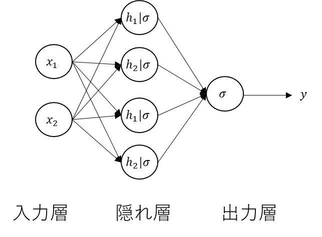
構造と数式【再掲】
隠れ層のユニットを増やした場合の構成を数式を再掲
\(
y=
\sigma\Bigg(
\begin{bmatrix}
w_{211}&w_{212}&w_{213}&w_{214}&b_2
\end{bmatrix}
\begin{bmatrix}
\sigma\bigg(
\begin{bmatrix}
w_{111}&w_{112}&b_1\\
w_{121}&w_{122}&b_1\\
w_{131}&w_{132}&b_1\\
w_{141}&w_{142}&b_1\\
\end{bmatrix}
\begin{bmatrix}
x_1\\x_2\\1
\end{bmatrix}
\bigg)\\
1
\end{bmatrix}
\Bigg)
\)
今回はこれをScilabで実現する。
Scilabコード
Scilabコードは以下。
// データの準備
X = [0 0; 0 1; 1 0; 1 1]; // 入力データ
Y = [0; 1; 1; 0]; // 出力データ

// シグモイド関数
function y = sigmoid(x)
    y = 1 ./ (1 + exp(-x));
endfunction

// シグモイド関数の導関数
function y = sigmoid_derivative(x)
    y = sigmoid(x) .* (1 - sigmoid(x));
endfunction

// ネットワークの構築
hidden_size = 4; // 隠れ層のユニット数
output_size = 1; // 出力層のユニット数
learning_rate = 0.5; // 学習率

input_size = size(X, 2);
W1 = rand(input_size, hidden_size, 'normal'); // 入力層から隠れ層への重み行列
b1 = rand(1, hidden_size, 'normal'); // 隠れ層のバイアス項
W2 = rand(hidden_size, output_size, 'normal'); // 隠れ層から出力層への重み行列
b2 = rand(1, output_size, 'normal'); // 出力層のバイアス項

// 学習
epochs = 4000; // エポック数

errors = zeros(epochs, 1); // エポックごとの誤差を保存する配列

for epoch = 1:epochs
    // 順伝播
    Z1 = X * W1 + ones(size(X, 1), 1) * b1; // 隠れ層の入力
    A1 = sigmoid(Z1); // 隠れ層の出力
    Z2 = A1 * W2 + b2; // 出力層の入力
    A2 = sigmoid(Z2); // 出力層の出力

    // 誤差計算(平均二乗誤差)
    error = (1 / size(X, 1)) * sum((A2 - Y).^2);
    errors(epoch) = error;

    // 逆伝播
    delta2 = (A2 - Y) .* sigmoid_derivative(Z2);
    delta1 = (delta2 * W2') .* sigmoid_derivative(Z1);

    grad_W2 = A1' * delta2;
    grad_b2 = sum(delta2);
    grad_W1 = X' * delta1;
    grad_b1 = sum(delta1);

    // パラメータの更新
    W1 = W1 - learning_rate * grad_W1;
    b1 = b1 - learning_rate * grad_b1;
    W2 = W2 - learning_rate * grad_W2;
    b2 = b2 - learning_rate * grad_b2;
end

// 決定境界線の表示
h = 0.01; // メッシュの間隔
[x1, x2] = meshgrid(min(X(:, 1)) - 0.5:h:max(X(:, 1)) + 0.5, min(X(:, 2)) - 0.5:h:max(X(:, 2)) + 0.5);
X_mesh = [x1(:) x2(:)];

hidden_layer_mesh = sigmoid(X_mesh * W1 + ones(size(X_mesh, 1), 1) * b1);
output_layer_mesh = sigmoid(hidden_layer_mesh * W2 + b2);
y_mesh = round(output_layer_mesh); // 出力を0または1に丸める

clf;
x = X_mesh(:, 1);
y = X_mesh(:, 2);

idx_boundary = find(y_mesh(1:$-1) <> y_mesh(2:$)); // 境界のインデックスを取得
boundary_x = x(idx_boundary); // 境界のx座標
boundary_y = y(idx_boundary); // 境界のy座標

scatter(boundary_x, boundary_y, 3, 'k', 'fill'); // 境界を黒でプロット
scatter(X(Y==0, 1), X(Y==0, 2), 100, 'r', 'fill');
scatter(X(Y==1, 1), X(Y==1, 2), 100, 'b', 'fill');
xlabel("X1");
ylabel("X2");
title("XOR Classification");
legend("Boundary", "Class 1", "Class 0");

xgrid; // グリッドの表示
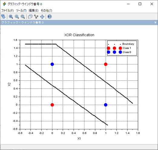
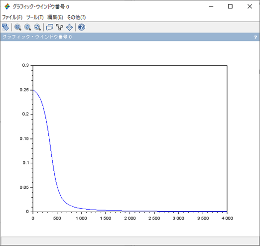
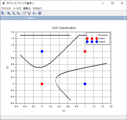
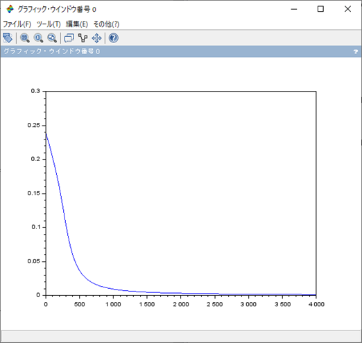
処理結果
処理結果は以下。
パターン2の方が隠れ層のユニット数を2から4にしたことで出てきた分類パターンになる。
パターン1
パターン2
まとめ
- 多層パーセプトロンの隠れ層のユニット数を2から4に変えたScilabコードで分類を実施。
- 大きく2パターンの分類パターンがある。
- やや複雑な分類パターンが4ユニットにすることで出てきたもの。
MATLAB、Python、Scilab、Julia比較ページはこちら
Pythonで動かして学ぶ!あたらしい線形代数の教科書

ゼロから作るDeep Learning ―Pythonで学ぶディープラーニングの理論と実装

ゼロからはじめるPID制御

OpenCVによる画像処理入門

恋する統計学[回帰分析入門(多変量解析1)] 恋する統計学[記述統計入門]

Pythonによる制御工学入門

理工系のための数学入門 ―微分方程式・ラプラス変換・フーリエ解析


コメント