
関数型プログラミングとの接点
関数型プログラミング(Functional Programming, FP)は、状態を持たない純粋関数を中心に構成される。この構造は、線形代数における「入力 → 出力」の写像と非常に近い。
高階関数と行列演算
関数型では、関数を引数に取る、あるいは関数を返す「高階関数」が基本的な構成要素となる。これは、行列を操作する関数やテンソル演算と構造的に一致する。
関数合成:
$$
f(x)=g(h(x)) \Leftrightarrow A\cdot(B\cdot x)=(A\cdot B)\cdot x
$$
この対応は、関数型の抽象的な処理の流れを線形代数的に明確に表現するものである。
例:高階関数の例(関数合成)
import numpy as np
import matplotlib.pyplot as plt

# --- 高階関数の例(関数合成) ---
def g(x):
    return x + 3

def f(x):
    return 2 * x + 5

# アフィン変換 g(x) = x + 3
A1 = np.array([[1]])
b1 = np.array([[3]])

# アフィン変換 f(x) = 2x + 5
A2 = np.array([[2]])
b2 = np.array([[5]])

# 拡張行列の構築(同次座標系)
A1_ext = np.hstack([A1, b1])           # [A1 | b1]
A1_ext = np.vstack([A1_ext, [0, 1]])   # 下に [0, 1] を追加

A2_ext = np.hstack([A2, b2])           # [A2 | b2]
A2_ext = np.vstack([A2_ext, [0, 1]])   # 下に [0, 1] を追加

# 合成変換行列 A_comp = A2_ext @ A1_ext
A_comp = A2_ext @ A1_ext

# 入力 x の範囲
x_vals = np.linspace(-10, 10, 200)
x_ext = np.vstack([x_vals, np.ones_like(x_vals)])  # 拡張ベクトル [x; 1]

# 各関数の出力
y_g = f(x_vals)
y_f = g(x_vals)
y_fg = f(g(x_vals))
y_comp = (A_comp @ x_ext)[0]  # 合成行列による出力

# グラフ描画
plt.figure(figsize=(10, 6))
plt.plot(x_vals, y_f, label='f(x) = 2x + 5', color='blue')
plt.plot(x_vals, y_g, label='g(x) = x + 3', color='orange')
plt.plot(x_vals, y_fg, label='f(g(x)) = 2(x + 3) + 5', linestyle='--', color='green')
plt.plot(x_vals, y_comp, label='Composition by augmented matrix', linestyle=':', color='red')

plt.title("Comparison of affine transformation synthesis and function synthesis")
plt.xlabel("x")
plt.ylabel("output ")
plt.grid(True)
plt.legend()
plt.tight_layout()
plt.show()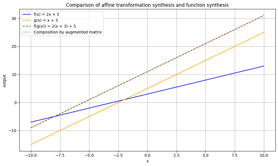
条件分岐の線形的表現と関数的抽象
関数型プログラミングでは、状態を持たず、条件分岐も関数として抽象化することが推奨される。これは、線形代数的な処理モデルと親和性が高い。
たとえば、従来の if 文による条件分岐は、明示的な制御構造であり、処理の流れを分岐させる。一方、ニューラルネットワークでは、ReLU や sigmoid のような非線形関数を用いて、条件分岐を連続的かつ微分可能な形で表現する。
このような非線形関数は、線形変換と組み合わせることで、複雑な振る舞いを滑らかに表現できる。さらに、関数型プログラミングにおけるパターンマッチや関数ディスパッチは、条件分岐の局所化と抽象化を実現し、ソフトウェアの構造を明快に保つ。
この構造は、以下のように整理できる:
| 概念 | ソフトウェア | 数理的対応 |
| 明示的条件分岐 | if, switch | 不連続な分岐 |
| 関数的抽象 | パターンマッチ、関数選択 | 関数合成、写像 |
| 数理的連続化 | ReLU, sigmoid | 非線形関数による滑らかな分岐 |
このように、条件分岐を関数として扱う発想は、線形代数的な処理モデルと関数型プログラミングの設計思想を橋渡しするものであり、抽象化の一形態として非常に有効である。
例:Haskellにおける階乗関数
factorial :: Integer -> Integer
factorial 0 = 1
factorial n = n * factorial (n - 1)
このように、条件分岐が関数定義の構造に組み込まれており、可読性と安全性が高まる。
import matplotlib.pyplot as plt
import numpy as np

# --- ① 従来型の条件分岐(if-else) ---
def factorial_if(n):
    if n == 0:
        return 1
    else:
        return n * factorial_if(n - 1)

# --- ② 関数型スタイル:辞書によるディスパッチ ---
def factorial_dispatch(n):
    dispatch = {
        0: lambda: 1  # n=0 の場合の処理
    }
    # 辞書に該当する関数があればそれを実行、なければ再帰的に計算
    return dispatch.get(n, lambda: n * factorial_dispatch(n - 1))()

# --- ③ パターンマッチ(Python 3.10以降) ---
def factorial_match(n):
    match n:
        case 0:
            return 1
        case _:  # その他の値
            return n * factorial_match(n - 1)

# --- 入力と出力の準備 ---
inputs = list(range(6))  # 0〜5までの整数
outputs_if = [factorial_if(n) for n in inputs]
outputs_dispatch = [factorial_dispatch(n) for n in inputs]
outputs_match = [factorial_match(n) for n in inputs]

# --- グラフ描画 ---
plt.figure(figsize=(10, 6))
plt.plot(inputs, outputs_if, label='if-else(conventional type)', marker='o')
plt.plot(inputs, outputs_dispatch, label='dictionary dispatch (functional)', marker='s')
plt.plot(inputs, outputs_match, label='match-case (pattern match)', marker='^')
plt.title("Factorial calculations with different conditional branching styles")
plt.xlabel("input value n")
plt.ylabel("factorial(n)")
plt.grid(True)
plt.legend()
plt.tight_layout()
plt.show()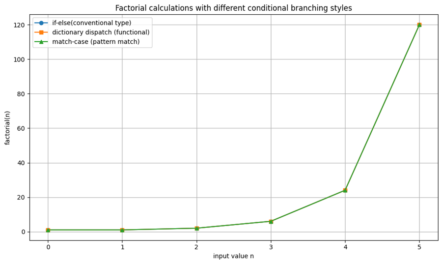

コメント