
MATLAB、Python、Scilab、Julia比較ページはこちら
https://www.simulationroom999.com/blog/comparison-of-matlab-python-scilab/

はじめに

の、
MATLAB,Python,Scilab,Julia比較 第2章 その41【二次形式の微分⑤】
を書き直したもの。
正規方程式を導出するまでの説明。
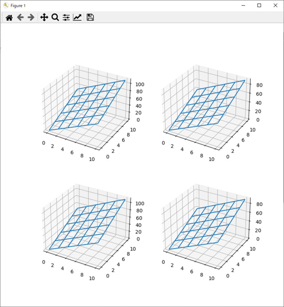
今回は二次形式の微分(勾配)を実際の多項式に適用したものをPython(NumPy)で算出&プロットしてみる。
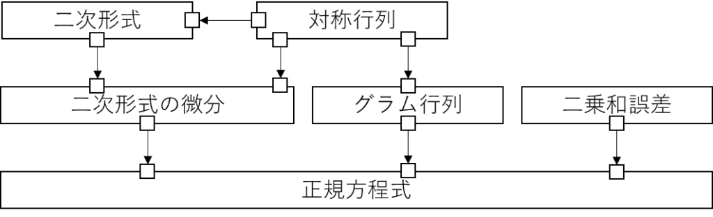
ロードマップ&数式【再掲】
まずはロードマップと数式を再掲。
二次形式の多項式
\(
f(x,y)=3x^2+2y^2+5xy
\)
二次形式の多項式の偏導関数
\(
\displaystyle\frac{\partial f(x,y)}{\partial x}=6x+5y
\)
\(
\displaystyle\frac{\partial f(x,y)}{\partial y}=4y+5x
\)
二次形式の行列形式の偏導関数
\(
\nabla f(x,y) =
\begin{bmatrix}
\displaystyle\frac{\partial f(x,y)}{\partial x} \\
\displaystyle\frac{\partial f(x,y)}{\partial y}
\end{bmatrix}=
2AX=2
\begin{bmatrix}
3 & 5/2 \\
5/2 & 2
\end{bmatrix}
\begin{bmatrix}
x \\
y
\end{bmatrix}
\)
今回はPython(NumPy)で計算。
Pythonコード
Pythonコードは以下になる。
import numpy as np
import matplotlib.pyplot as plt

a=3
b=2
c=5
A=np.array([[a,c/2],[c/2,b]])

N=6
ax=np.linspace(0,10,N)
ay=np.linspace(0,10,N)
x,y=np.meshgrid(ax,ay)

fig = plt.figure(figsize=(8, 8))

polyY1=6*x+5*y
polyY2=5*x+4*y
ax = fig.add_subplot(2, 2, 1, projection='3d')
ax.plot_wireframe(x,y,polyY1)
ax = fig.add_subplot(2, 2, 2, projection='3d')
ax.plot_wireframe(x,y,polyY2)

X=np.block([[x.reshape(-1)],[y.reshape(-1)]])
Y=2*A@X
matY1=Y[0].reshape(N,N)
matY2=Y[1].reshape(N,N)
ax = fig.add_subplot(2, 2, 3, projection='3d')
ax.plot_wireframe(x, y, matY1)
ax = fig.add_subplot(2, 2, 4, projection='3d')
ax.plot_wireframe(x, y, matY2)

plt.show()

print("polyY1=")
print(polyY1)
print("polyY2=")
print(polyY2)
print("matY1=")
print(matY1)
print("matY2=")
print(matY2)
処理結果
そして処理結果。
polyY1=
[[  0.  12.  24.  36.  48.  60.]
 [ 10.  22.  34.  46.  58.  70.]
 [ 20.  32.  44.  56.  68.  80.]
 [ 30.  42.  54.  66.  78.  90.]
 [ 40.  52.  64.  76.  88. 100.]
 [ 50.  62.  74.  86.  98. 110.]]
polyY2=
[[ 0. 10. 20. 30. 40. 50.]
 [ 8. 18. 28. 38. 48. 58.]
 [16. 26. 36. 46. 56. 66.]
 [24. 34. 44. 54. 64. 74.]
 [32. 42. 52. 62. 72. 82.]
 [40. 50. 60. 70. 80. 90.]]
matY1=
[[  0.  12.  24.  36.  48.  60.]
 [ 10.  22.  34.  46.  58.  70.]
 [ 20.  32.  44.  56.  68.  80.]
 [ 30.  42.  54.  66.  78.  90.]
 [ 40.  52.  64.  76.  88. 100.]
 [ 50.  62.  74.  86.  98. 110.]]
matY2=
[[ 0. 10. 20. 30. 40. 50.]
 [ 8. 18. 28. 38. 48. 58.]
 [16. 26. 36. 46. 56. 66.]
 [24. 34. 44. 54. 64. 74.]
 [32. 42. 52. 62. 72. 82.]
 [40. 50. 60. 70. 80. 90.]]
考察
結果としてはMATLABと同じく完全一致。
計算としては全く一緒で、演算誤差が出るような計算でもない。
まとめ
- 二次形式の多項式としての偏導関数、行列形式による偏導関数を元にPython(NumPy)で算出及びプロット。
- ともに同一の算出結果とプロットが得られた。
MATLAB、Python、Scilab、Julia比較ページはこちら


コメント