
MATLAB、Python、Scilab、Julia比較ページはこちら
https://www.simulationroom999.com/blog/comparison-of-matlab-python-scilab/

はじめに

の、
MATLAB,Python,Scilab,Julia比較 第3章 その42【非極大値抑制⑦】
非極大値抑制をプログラムで実現してみる。
今回はPython(NumPy)で実施。
動作確認用処理【再掲】
まずは、非極大値抑制の実験の処理手順を再掲
- Sobelフィルタ等の微分フィルタで以下を推定
- x軸、y軸の濃淡変化量
- 変化強度(ノルム)
- 「x軸、y軸の濃淡変化量」から勾配方向角を推定
- arntan関数を利用
- 勾配方向を垂直(UD)、水平(LR)、斜め右上から右下(RULD)、斜め左上から右下の4パターンに丸め。
- 勾配方向角に応じて極大値評価をして非極大値だったら「変化強度(ノルム)」 を0値埋め
- 画像出力
これをPython(NumPy)で実現する。
Pythonコード
Pythonコードは以下になる。
import numpy as np
import cv2


# 畳み込み演算
def convolution2d(img, kernel):
    m, n = kernel.shape # カーネルサイズ取得

    # カーネル中心からみた幅
    dy = int((m-1)/2)  # カーネル上下幅
    dx = int((n-1)/2)  # カーネル左右幅

    h, w = img.shape   # イメージサイズ
    out = np.zeros((h, w)) # 出力用イメージ

    # 畳み込み
    for y in range(dy, h - dy):
        for x in range(dx, w - dx):
            out[y][x] = np.sum(img[y-dy:y+dy+1, x-dx:x+dx+1]*kernel)

    return out

# Non maximum Suppression
def non_maximum_suppression(G, theta):
    h, w = G.shape
    out = G.copy()

    # 勾配方向を4方向(LR,UD,RULD,LURD)に近似
    theta[np.where(( -22.5 <= theta) & (theta <   22.5))] = 0   # LR    ─
    theta[np.where((  22.5 <= theta) & (theta <   67.5))] = 45  # RULD  /
    theta[np.where((  67.5 <= theta) & (theta <  112.5))] = 90  # UD    │
    theta[np.where(( 112.5 <= theta) & (theta <  157.5))] = 135 # LURD  \
    theta[np.where(( 157.5 <= theta) & (theta <  180.0))] = 0   # LR    ─
    theta[np.where((-180.0 <= theta) & (theta < -157.5))] = 0   # LR    ─
    theta[np.where((-157.5 <= theta) & (theta < -112.5))] = 45  # RULD  /
    theta[np.where((-112.5 <= theta) & (theta <  -67.5))] = 90  # UD    │
    theta[np.where(( -67.5 <= theta) & (theta <  -22.5))] = 135 # LURD  \

    # 現画素の勾配方向に接する2つの画素値を比較し、現画素が極大値でなければ0にする。
    for y in range(1, h - 1):
        for x in range(1, w - 1):
            if theta[y][x] == 0:    # LR    ─
                if (G[y][x] < G[y][x+1]) or (G[y][x] < G[y][x-1]):
                    out[y][x] = 0
            elif theta[y][x] == 45: # RULD  /
                if (G[y][x] < G[y-1][x+1]) or (G[y][x] < G[y+1][x-1]):
                    out[y][x] = 0
            elif theta[y][x] == 90: # UD    │
                if (G[y][x] < G[y+1][x]) or (G[y][x] < G[y-1][x]):
                    out[y][x] = 0
            else:                   # LURD  \
                if (G[y][x] < G[y+1][x+1]) or (G[y][x] < G[y-1][x-1]):
                    out[y][x] = 0
    return out

def non_maximum_suppression_test():
    # 入力画像の読み込み
    img = cv2.imread("dog.jpg")
    b = img[:,:,0]
    g = img[:,:,1]
    r = img[:,:,2]

    # ガウシアンフィルタ用のkernel
    kernel_gauss = np.array([[1/16, 2/16, 1/16],
                             [2/16, 4/16, 2/16],
                             [1/16, 2/16, 1/16]])
    # Sobelフィルタ用のKernel
    kernel_sx = np.array([[-1,  0,  1],
                          [-2,  0,  2],
                          [-1,  0,  1]])
    kernel_sy = kernel_sx.T

    # SDTVグレースケール
    gray_sdtv = np.array(0.2990 * r + 0.5870 * g + 0.1140 * b, dtype='uint8')

    # ガウシアンフィルタ
    img_g = convolution2d(gray_sdtv, kernel_gauss)

    # Sobelフィルタ
    Gx = convolution2d(img_g, kernel_sx)
    Gy = convolution2d(img_g, kernel_sy)

    # 勾配強度と角度
    G = np.sqrt(Gx**2 + Gy**2)
    theta = np.arctan2(Gy, Gx) * 180 / np.pi
    cv2.imwrite("dog_nms_G.jpg",np.abs(G)) # 255オーバーあり
    cv2.imwrite("dog_nms_theta.jpg",np.abs(theta)) # -180~180

    # 極大値以外を除去(Non maximum Suppression)
    G_nms = non_maximum_suppression(G, theta)
    cv2.imwrite("dog_nms.jpg",G_nms) # 255オーバーあり

    return

non_maximum_suppression_test()
処理結果
そして処理結果。
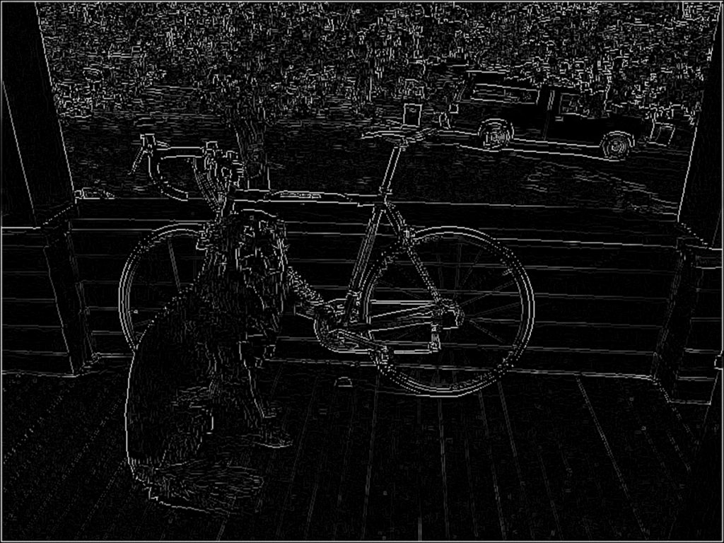
考察
これもMATLABと同じ結果が得られた。
(演算が一緒だから当たり前ではあるが・・・。
気になる点と言えばコード上のこれ。
theta[np.where(( -22.5 <= theta) & (theta < 22.5))] = 0線形インデックスサーチになる。
MATLABでやったときは論理インデックスサーチを使用していたが、
今回はあえて線形インデックスサーチにしてみた。
ちなみに、論理インデックスサーチ、線形インデックスサーチは
MATLAB,Python(NumPy)ともに実施可能。
まとめ
- Python(NumPy)で非極大値抑制を実施。
- MATLABと同一の結果が得られた。
- MATLABでは論理インデックスサーチを使用したが、ここではあえて線形インデックスサーチを使用。
MATLAB、Python、Scilab、Julia比較ページはこちら


コメント